Overview of generative models
Normalizing Flows
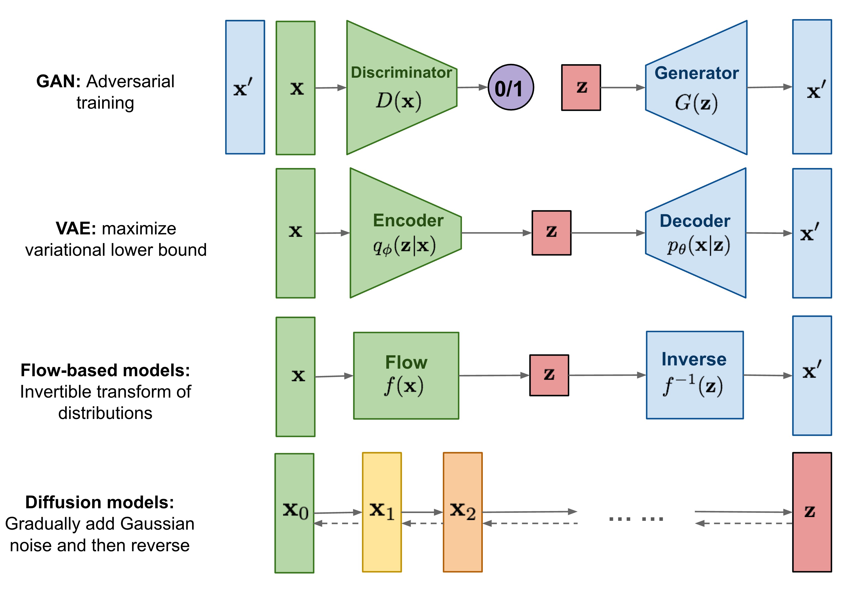
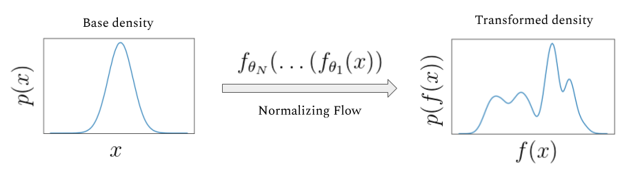
Normalizing Flows (NFs) (Rezende & Mohamed, 2015) learn an invertible mapping from an (easy) latent/base/source distribution to a given data/target distribution.
n_samples = 1000
target_data, _ = datasets.make_circles(n_samples=n_samples, factor=0.5, noise=0.05)
target_data = StandardScaler().fit_transform(target_data)

plt.scatter(target_data[:,0], target_data[:,1], alpha=0.5)
plt.show()

Let us take a standard normal as a latent distribution.
latent_dist = torch.distributions.Independent(torch.distributions.Normal(torch.zeros(2), torch.ones(2)), 1)

latent_data = latent_dist.sample(torch.Size([1000,])).detach().numpy()
plt.scatter(latent_data[:,0], latent_data[:,1], color=sns.color_palette()[1], alpha=0.5)
plt.show()

Now we map samples from the base distribution through a neural network and look at the output.
bijector = bijectors.SplineAutoregressive()
transformed_dist = distributions.Flow(latent_dist, bijector)

data = transformed_dist.sample(torch.Size([1000,])).detach().numpy()
plt.scatter(data[:,0], data[:,1], color=sns.color_palette()[2], alpha=0.5)
plt.show()

Let us optimize the neural network by maximing the log-likelihood of the data samples.
dataset = torch.tensor(target_data, dtype=torch.float)
optimizer = torch.optim.Adam(transformed_dist.parameters(), lr=5e-3)
for step in range(2000):
    optimizer.zero_grad()
    loss = -transformed_dist.log_prob(dataset).mean()
    loss.backward()
    optimizer.step()

    if step % 500 == 0:
        print('step: {}, loss: {}'.format(step, loss.item()))
step: 0, loss: 2.885023355484009
step: 500, loss: 1.8666640520095825
step: 1000, loss: 1.8461662530899048
step: 1500, loss: 1.7394717931747437
data = transformed_dist.sample(torch.Size([1000,])).detach().numpy()
plt.scatter(target_data[:,0], target_data[:,1], alpha=0.5, label="data")
plt.scatter(data[:,0], data[:,1], color=sns.color_palette()[2], alpha=0.5, label="prediction")
plt.legend()
plt.show()

This looks pretty good!
But how did we compute the log-likelihood transformed_dist.log_prob(dataset)?
Theoretical foundations
Let us start with a more formal definition:
- $X$ ... random variable (with density $ p_{X}$) describing the data distribution
- $Z$ ... random variable (with density $ p_{Z}$) describing the latent distribution
Normalizing flows deal with parametrized, measurable mappings $f_\theta$, which transform a base distribution $ p_{Z}$ into a target distribution $ p_{X}$.
In other words, we seek a transformation $f_\theta$ such that the random variable
\begin{equation*} X_\theta := f_\theta(Z) \quad \text{(with density } p_{X_\theta}) \end{equation*}satisfies $ p_{X_\theta} \approx p_{X}$.
Question: How can we compute the log-likelihood $\log p_{X_{\theta}}(X)$ of our data $X$ under our (parametrized) model $p_{X_{\theta}}$?
Tool 1: Change of variables formula
For a diffeomorphism $f_\theta$ it holds that
\begin{equation*} p_{X_\theta} = \left( p_{Z} \circ f_\theta^{-1} \right) | \det (\nabla f_\theta^{-1})|. \end{equation*}This implies that
\begin{equation*} \log p_{X_{\theta}}(X) = \log \left( p_{Z} \circ f_\theta^{-1} \right)(X) + \log | \det (\nabla f_\theta^{-1}(X))|. \end{equation*}Choosing a tractable latent distribution $Z$ (such as a Gaussian), we can evaluate $p_Z$.
Thus, we seek mappings $f_\theta$ where we can (efficiently) compute the inverse $f_\theta^{-1}$ and the Jacobian determinant $\det (\nabla f_\theta^{-1})$.
Tool 2: Closedness of diffeomorphisms under compositions
For diffeomorphisms $f^{(1)}$ and $f^{(2)}$ it holds that
\begin{equation*} \left(f^{(2)}\circ f^{(1)}\right)^{-1} = (f^{(1)})^{-1} \circ (f^{(2)})^{-1} \end{equation*}and \begin{equation*} \det\left(\nabla \left(f^{(2)}\circ f^{(1)}\right)\right) = \det\left( \left(\nabla f^{(2)}\right) \circ f^{(1)}\right) \det\left(\nabla f^{(1)}\right). \end{equation*}
Therefore, we can focus our attention on the construction of rather simple transformations $f_\theta^{(\ell)}$ which can then be composed, i.e.,
\begin{equation*} f_\theta = f^{(L)}_\theta \circ \dots \circ f^{(1)}_\theta. \end{equation*}E.g., the so-called Glow architecture has $L=320$ sub-transformations.

Brief summary
- $f_\theta = f^{(L)}_\theta \circ \dots \circ f^{(1)}_\theta$
- each $f^{(\ell)}_\theta$ is a diffeomorphism with parameters $\theta$
- base distribution $Z$ is taken to be simple distribution (such as a multivariate Gaussian)
Normalizing flows allow us to
- sample from $p_{X_\theta}$ via $$X=f_\theta(Z)$$
given that we can sample from $p_{Z}$ and evaluate $f_\theta$.
- evaluate the density $p_{X_\theta}$ via
given that we can evaluate the density $p_{Z}$, evaluate the inverse $f_ \theta^{-1}$, and its Jacobian determinant $\det(\nabla f_ \theta^{-1})$.
The term normalizing flow refers to the trajectory through $(f_\theta^{(L)})^{-1}, \dots, (f_\theta^{(1)})^{-1}$ that a sample from $X_\theta = f_\theta(Z)$ follows as it is transformed (normalized) into a sample from the (simple) latent distribution $Z$.
Remarks on the objective
- log-likelihood training/forward KL-divergence:
- needs data $(X^{(i)})_{i=1}^m$ and evaluation and differentiation of $f_\theta^{-1}$, its Jacobian determinant, and $p_{Z}$:
Reverse KL-divergence (sampling from unnormalized densities):
- needs data $(Z^{(i)})_{i=1}^m$ and evaluation and differentiation of $f_\theta$, its Jacobian determinant, and the unnormalized density $C \cdot p_{X}$:
\begin{equation*} D_{\textrm{KL}}(X_\theta \parallel X ) = \underbrace{\mathbb{E}\left[ \log p_{Z}(Z)\right]}_{\text{const.}} - \mathbb{E}\left[ \log\big| \det( \nabla f_\theta(Z))\big| \right] - \mathbb{E}\left[ \log\big(C\cdot p_{X}(f_\theta(Z))\big)\right] + \underbrace{\log\big(C \big)}_{\text{const.}}. \end{equation*}
Some architectures
(Of course) we parametrize $f^{(\ell)}_\theta$ as neural networks:
Jacobian of $\nabla f^{(\ell)}_\theta$ can always be obtained by $d$ backward passes and its determinant can be computed with $\mathcal{O}(d^3)$ flops.
We seek methods for which the complexity of computing the Jacobian determinant scales only linearly in the data dimension $d$.
![Overview from [Papamakarios et al., 2021]](flow_overview.png)
Autoregressive Flows
- Composed of functions of the form \begin{equation*} f_\theta(x) = \big(\tau_{c_i}(x_i)\big)_i \quad \text{with} \quad c_i = c^{(i)}_\theta(x_{i-1},\dots,x_1). \end{equation*}
- The conditioner $c^{(i)}_\theta$ parametrizes the univariate transformer $\tau_{c}$.
- For every $c$ the transformer $\tau_{c}$ is assumed to be monotonic and thus invertible.
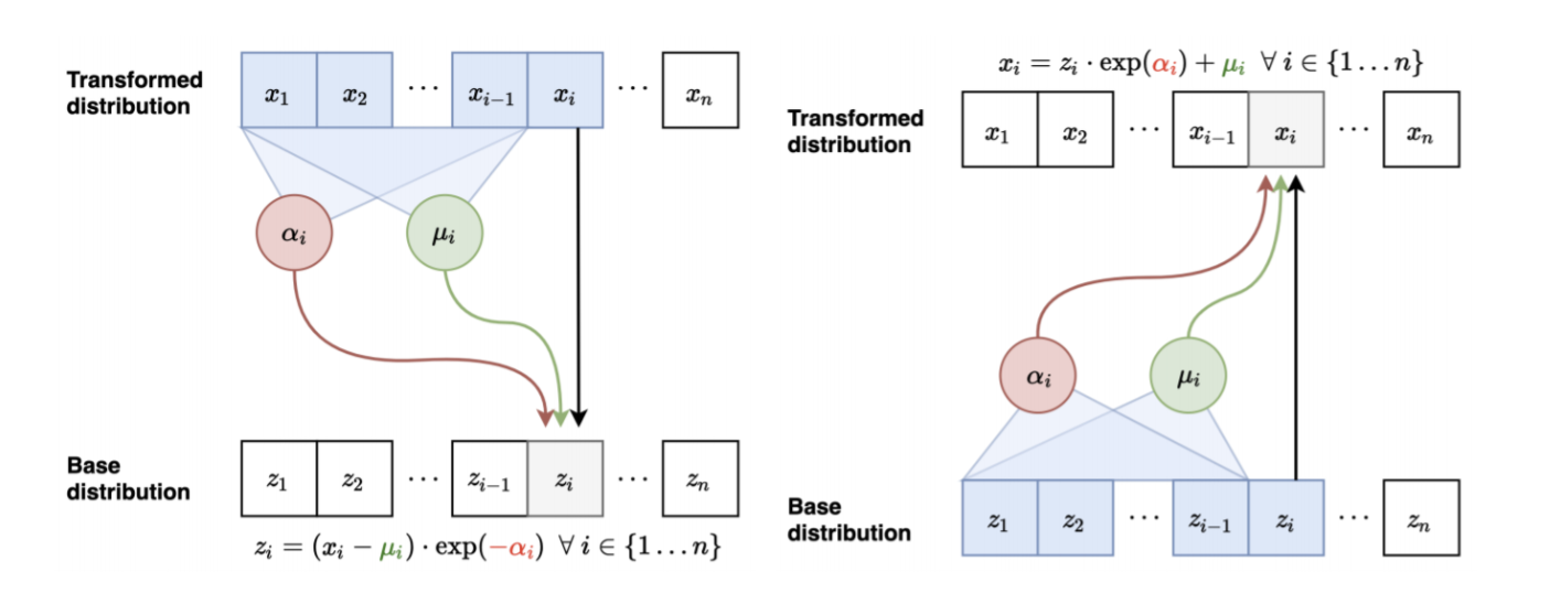
$\Rightarrow$ represent the inverse and the Jacobian determinant as \begin{equation*} f^{-1}_\theta(y) = \big(\tau^{-1}_{c_i}(y_i)\big)_i \quad \text{and} \quad \det(\nabla f_\theta(x)) = \prod_{i=1}^d \tau'_{c_i}(x_i). \end{equation*}
Transformers $\tau_c$:
- affine functions (limited expressivity)
- compositions or conic combinations of monotonic functions (might need iterative methods to be inverted, e.g., bisection search)
- integrals of strictly positive functions (need numerical approximation or special integrands, e.g. polynomials; typically not analytically invertible)
- splines with parametrized knots (invertibility is guaranteed by invertibility of each piece where the index can be found efficiently by binary search)

Conditioners $c_i$: Efficient conditioners should share parameters across the $d$ conditioners $(c_\theta^{(i)})_{i=1}^d$ and viable options include:
- recurrent neural networks (requires to compute $(c_i)_i$ iteratively)
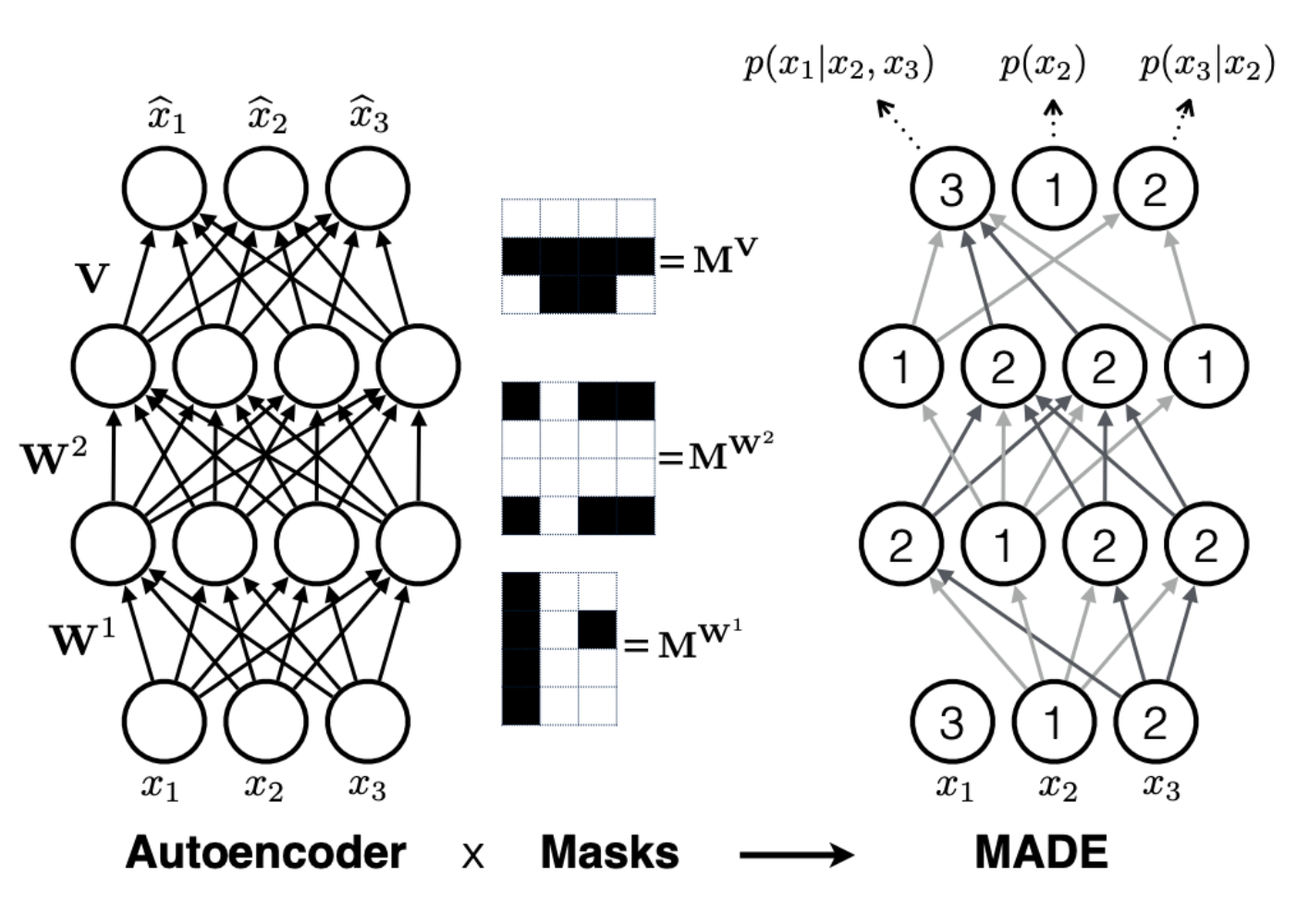
- masked neural networks where the index set $I=\{1,\dots,d\}$ is filtered into $K$ parts $I_1 \subset \dots \subset I_k=I$ and connections are masked such that the output $(c_i)_{i\in I_k \cap I_{k-1}}$ only depends on $(x_i)_{i\in I_{k-1}}$
- outputs all $(c_i)_i$ at once
- inverse flow needs $\mathcal{O}(K)$ forward passes until all coordinates of $x$ are known
- $K$ trades off expressivity for efficiency ($K=d$ yields a fully auto-regressive structure, $K=2$ is called a coupling layer)
- $(c^{(i)}_\theta)_{i\in I_1}$ sometimes chosen to be the identity.
Linear Flows
Autoregressive flows depend on the order of the input coordinates (for masked NNs with $K<d$ not all coordinates interact with each other).
$\Rightarrow$ use permutations or, more general, invertible matrices as parts of the flow, i.e.,
\begin{equation*} f_\theta(x) := W_\theta x \quad \text{with} \quad W_\theta \in \mathbb{R}^{d\times d} \quad \text{and} \quad \det(W_\theta) \in \mathbb{R}\setminus \{0\}. \end{equation*}Naive implementations need $\mathcal{O}(d^3)$ flops to invert $W_\theta$ or compute $\det(W_\theta)$.
$\Rightarrow$ use structured families of matrices $(W_\theta)_\theta$, e.g. triangular matrices with its diagonal elements reparametrized by $e^{\theta_i}$ to guarantee positivity.
Residual Flows
Building blocks of the form \begin{equation*} f_\theta(x) := x + g_\theta(x), \end{equation*} where $g_\theta$ is based on:
Contractions
- iterative inversion using the Banach fixed-point theorem.
- estimate of the logarithm of the absolute Jacobian determinant using the Maclaurin series
\begin{equation*} \log \left| \det(\nabla f_\theta) \right| = \sum_{k=1}^\infty \frac{(-1)^{k+1}}{k} \operatorname{tr}\left((\nabla g_\theta)^k\right) \approx \sum_{k=1}^\infty \frac{(-1)^{k+1}}{k} v^\top \left((\nabla g_\theta)^k\right) v, \end{equation*}
where $v\in\mathbb{R}^d$ is a sample of a distribution with zero mean and covariance matrix $I_d$ (Hutchinson trace estimator).
Matrix determinant lemma: \begin{equation*} \det(\nabla f_\theta) = \det(A+VW^\top) = \det(I_d+W^\top A^{-1}V)\det(A) \end{equation*}
- efficient Jacobian determinant
- no analytical inverse $\Rightarrow$ mostly used to approximate posteriors
Universality
One-dimensional case: the probability integral transform and inverse transform sampling ensure that
\begin{equation*} F_X(X) \sim U \quad \text{and} \quad F_X^{-1}(U) \sim X, \quad \text{where} \quad U\sim \mathcal{U}([0,1]). \end{equation*}$F_X$ is the cumulative distribution function (CDF) and $F_X^{-1}$ its generalized inverse given by
\begin{equation*} F_X^{-1}(y) = \inf \{ x \colon F_X(x) \le y \}, \quad y\in (0,1). \end{equation*}$\Rightarrow$ $f_\theta:=F_X^{-1} \circ F_{Z}$ satisfies $ f_\theta(Z_\theta) \sim X$ yielding a suitable transformation.
Multi-dimensional case: Under suitable regularity conditions, a similar statement can be established by considering the CDFs of the conditionals, i.e.,
\begin{align} F^{(i)}_X(x_i, \dots, x_1) &= \mathbb{P}\left[X_i \le x_i | (X_{i-1}=x_{i-1}, \dots, X_1=x_1)\right] \\ &=\int_{-\infty}^{x_i} p_{X_i | (X_{i-1}, \dots, X_1)}(\xi | x_{i-1}, \dots, x_1) \mathrm{d}\xi. \end{align}$\Rightarrow$ autoregressive flows are universal.
Some comparsions
... to diffusion models on Cifar and ImageNet:

Apart from generation, interesting applications include: density estimation, auxiliary distributions for importance sampling, proposals for MCMC, approximation of posteriors, ...
Final remarks on continuous-time normalizing flows
Viewing $\ell$ as discretization of a continuous time variable $t$, we can describe continuous-time flows using ODEs of the form \begin{equation*} \frac{ \mathrm{d} Z^{(t)}_\theta}{\mathrm{d}t} = g_\theta (t, Z^{(t)}_\theta) \quad \text{with} \quad Z^{(0)}_\theta = Z. \end{equation*}
The change in log density can also be described by an ODE, i.e.,
\begin{equation*} \frac{ \mathrm{d} \log \big( p_{Z^{(t)}_\theta} \big)}{\mathrm{d}t} = - \operatorname{tr} \left(\nabla g_\theta (t, \cdot) \right), \end{equation*}where the trace can be estimated using Hutchinson's trace estimator in a single backward pass.
- no other requirements to compute the change in density or to be invertible (i.e., running the ODE backwards).
- all intermediate spaces need to be homeomorphic $\Rightarrow$ topological constraints.